Exploring Swarm Dynamics with Multi-Agent Reinforcement Learning

Multi-Agent Environment

During my internship in Computational Neuroscience for my Master 2 at Inserm, I worked on Human-Robot Cooperation (HRC) under the supervision of Pr. Peter Ford Dominey, where a human and a robot were agents cooperating toward a common goal.

It was a great experience, and working with a real-world robotic platform was super exciting. But I’ve always wanted to explore what happens when you introduce more agents into the same environment. How do they interact? How do they learn from each other?

First, the environment becomes non-stationary: from the perspective of a single agent, the world becomes harder to predict, requiring agents to adapt to evolving situations as the other agents are simultaneously learning and changing their own behaviors.

I recently discovered MADDPG (Multi-Agent Deep Deterministic Policy Gradient), a popular reinforcement learning (RL) algorithm introduced by Lowe et al. in 2017, which is quite more recent (my internship was in 2009, don’t judge me!).

In this post, we’ll apply this algorithm on a small sandbox environment and explore the MADDPG behavior across progressively more complex simulations. We’ll walk through:

The Theory: The core concepts of MADDPG (Centralized Training, Decentralized Execution).
The Environment: The underlying Multi-Agent Particle Environment.
The Implementation: A deep dive into the code (MLP architectures, Gumbel-Softmax differentiable sampling, and stable Bellman updates via Target Networks).
The Experiments: A summary of our 10 incremental scenarios, accompanied by animations of the learned behaviors.
Learnings & Conclusion: Our key takeaways, mathematical insights on reward shaping, and macOS Apple Silicon compatibility adjustments.

1. The Theory: How MADDPG Works

Standard Actor-Critic methods (like the original Deep Deterministic Policy Gradient, or DDPG; see Lillicrap et al. in 2015) use two neural networks per agent:

An Actor (denoted as $\pi(o) \rightarrow a$) that decides the best action $a$ to take given the current observation $o$. It controls the agent.
A Critic (denoted as $Q(o, a) \rightarrow v$) that evaluates how good that action $a$ was afterward. It evaluates the actor’s actions.

Environment

Actor Network

Actor

• Policy $\pi(o)$
• Maps observation $o$ to action $a$

Action
$a$

Critic Network

Critic

• Evaluates $Q(o, a)$
• Takes observation & action

Action-value
$v$

Local Observation. The Actor and the Critic both observe the local state $o$ from the environment.

Decentralized Execution. The Actor maps the observation $o$ to an action $a = \pi(o)$, executing it in the environment.

Critic Evaluation. The Critic network receives the chosen action $a$ along with the observation $o$ to evaluate it.

Value Estimation. The Critic outputs the estimated action-value $Q(o, a)$ assessing the quality of the action.

Policy Gradient Update. The value gradient from the Critic is backpropagated to update the Actor's policy parameters $\nabla \pi$.

While powerful, these methods struggle in multi-agent settings because each agent only observes its own local environment. To fix this, MADDPG proposes a clever approach: Centralized Training with Decentralized Execution.

Central
Environment

Agent 1 Actor

Actor 1

• Policy $\pi_1(o_1)$
• Maps local observation $o_1$ to action $a_1$

Action $a_1$

Agent 2 Actor

Actor 2

• Policy $\pi_2(o_2)$
• Maps local observation $o_2$ to action $a_2$

Action $a_2$

Centralized Critics (Centralized Training)

Centralized Critic 1

• Evaluates $Q_1(o_1, o_2, a_1, a_2) \rightarrow v_1$
• Takes joint observations and actions

Centralized Critic 2

• Evaluates $Q_2(o_1, o_2, a_1, a_2) \rightarrow v_2$
• Takes joint observations and actions

Local Observations. Each agent $i$ independently receives its own local observation $o_i$ from the environment.

Decentralized Execution. Each Actor network maps its local observation to an action $a_i$ and executes it in the environment.

Centralized Training (Observations). During training, the Centralized Critics receive the joint observations $(o_1, o_2)$ of all agents.

Action Evaluation. Each Centralized Critic receives the action of its corresponding agent.

Action Sharing. The Centralized Critics also receive actions of all other agents (e.g., $a_1$ shared to Critic 2, $a_2$ shared to Critic 1) to restore environmental stationarity.

Policy Gradient Update. The Centralized Critics evaluate the joint actions/observations and backpropagate the policy gradients ($\nabla \pi_1, \nabla \pi_2$) to update their respective Actor policies.

Why does this matter? In a multi-agent environment, if agent $i$ only looks at its own action $a_i$ (like in standard single-agent DDPG), the transition dynamics of its local observation look like: $P(o'_i \mid o_i, a_i)$.

This transition probability changes over time because the other agents are also changing their behaviors as they learn. This is what makes the environment non-stationary and hard to learn.

However, if the Critic has access to the observations and actions of all agents, the transitions are governed by the joint observation physics: $P(o'_1, \dots, o'_N \mid o_1, \dots, o_N, a_1, \dots, a_N)$.

Since the physics of the environment do not change, this joint transition probability is stationary (constant), allowing the Critic to learn stable value estimates even while all agents’ policies are changing simultaneously.

Decentralized Execution (The Actor): The Actor network $\pi(o) \rightarrow a$ still only relies on local observations $o_i$ during execution. Once deployed, the agents act independently based on what they can see, without needing a global view.

2. The Environment: Multi-Agent Particle Environments

The Playground: OpenAI’s Multi-Agent Particle Environments (MPE). To test this, we use a custom sandbox based on OpenAI’s Multi-Agent Particle Environments. It features a simple 2D particle world with continuous observations and continuous/discrete action spaces, complete with basic simulated physics (such as momentum, friction, and elastic collisions).

Circle Sandbox Environment

In this sandbox, agents can move around, push each other, and navigate to various dynamic landmarks or follow other target agents in complex formations.

The input observation ($o$) of an agent in an environment can be computed from the environment state $s$, which contains at any given time:

The different entities’ positions and velocities.
Whether landmarks are active or not.
We created helper functions to easily compute the observation (select active landmarks, an agent, etc.).

The output action ($a$) is a vector of 5 logits: [No action, Right, Left, Up, Down]. This is converted by the environment into a 2D force vector applied to the agent in environment.py:

if self.discrete_action_space:
    # action[0][1] is Right, action[0][2] is Left
    agent.action.u[0] += action[0][1] - action[0][2]
    # action[0][3] is Up, action[0][4] is Down
    agent.action.u[1] += action[0][3] - action[0][4]
else:
    agent.action.u = action[0]
sensitivity = 5.0
if agent.accel is not None:
    sensitivity = agent.accel
agent.action.u *= sensitivity

We also modified the physics to have a stronger collision repulsion parameter:

In the World constructor in core.py:

# contact response parameters (add stronger collision response: 100 -> 500)
self.contact_force = 5e2

Applied in the World’s get_collision_force, still in core.py:

def get_collision_force(self, entity_a, entity_b):
    if (not entity_a.collide) or (not entity_b.collide):
        return [None, None]
    if entity_a is entity_b:
        return [None, None]
    
    # Calculate distance and overlap threshold
    delta_pos = entity_a.state.p_pos - entity_b.state.p_pos
    dist = np.sqrt(np.sum(np.square(delta_pos)))
    dist_min = entity_a.size + entity_b.size
    
    # Softmax penetration depth calculation
    k = self.contact_margin
    penetration = np.logaddexp(0, -(dist - dist_min) / k) * k
    
    # Repulsion force vector
    force = self.contact_force * delta_pos / dist * penetration  # <-- Repulsion calculation using the contact_force
    
    force_a = +force if entity_a.movable else None
    force_b = -force if entity_b.movable else None
    return [force_a, force_b]

Let’s now see how all these pieces come together. You can skip Section 3 if you are not interested in the implementation details. In this case, let’s meet in Section 4 to see the results :)

3. Digging into the implementation

To see how these concepts map to actual code, let’s explore the core implementation of the MADDPG algorithm located in maddpg.py and the training scripts.

3.1. Neural Network Architectures

Both the Actor and the Critic networks share a Multi-Layer Perceptron (MLP) architecture layout defined in train.py:

def mlp_model(input, num_outputs, scope, reuse=False, num_units=64, rnn_cell=None):
    with tf.compat.v1.variable_scope(scope, reuse=reuse):
        out = input
        out = layers.fully_connected(
            out, num_outputs=num_units, activation_fn=tf.nn.relu
        )
        out = layers.fully_connected(
            out, num_outputs=num_units, activation_fn=tf.nn.relu
        )
        out = layers.fully_connected(out, num_outputs=num_outputs, activation_fn=None)
        return out

For each agent $i$, the model instantiates two networks:

3.1.1. Actor Network (Policy / $\pi(o_i) \rightarrow a_i$)

Input: The agent’s own local observation vector $o_i$ (e.g., dimension is 7 for Experiment 8).
Hidden Layers: 2 fully connected (dense) layers of size 64 (num_units=64) with ReLU activations.
Output: A fully connected layer outputting raw logits of size equal to the action space dimension (e.g., 5 for discrete movements: [No action, Right, Left, Up, Down]). These logits are subsequently passed to a Gumbel-Softmax distribution to sample action vectors.

3.1.2. Critic Network (Q-Value / $Q_i(o_1, \dots, o_N, a_1, \dots, a_N) \rightarrow v$)

Input: Concatenation of the observations and actions of all $N$ agents in the environment: $\text{Input}_{\text{critic}} = [o_1, \dots, o_N, a_1, \dots, a_N]$ For example, with 4 agents in Experiment 8, the input size is $(4 \times 7) + (4 \times 5) = 48$ elements.
Hidden Layers: 2 layers of size 64 (num_units=64) with ReLU activations.
Output ($v$): A single unit (dimension 1) output representing the predicted action-value $Q(o, a)$ (linear activation).

3.2. Actor Training & Action Sampling

The Actor network’s job is to select the best action given only local observations. The training setup is constructed in p_train inside maddpg.py:

3.2.1. Action Selection & Gumbel-Softmax

The Actor network (p_func) outputs logits for actions. To make the action selection both stochastic (for exploration) and differentiable (so gradients can flow back), MADDPG wraps logits in a Gumbel-Softmax distribution:

# Build raw logits using the actor model
p = p_func(p_input, int(act_pdtype_n[p_index].param_shape()[0]), scope="p_func", num_units=num_units)
# Wrap parameters in a Gumbel-Softmax distribution
act_pd = act_pdtype_n[p_index].pdfromflat(p)
# Sample action
act_sample = act_pd.sample()

Differentiable Action Sampling: The Gumbel-Softmax

To train the Actor, we must calculate the gradient of the Critic’s evaluation with respect to the chosen action, and propagate it back into the Actor’s parameters. This poses a “small” challenge: we need the actions to be differentiable during training, but discrete during execution so that the agent actually takes actions. Let’s compare three common solutions: the standard Softmax, a Random Discrete Sampling, and the one used in this implementation: the Gumbel-Softmax trick.

Standard Softmax: Maps raw logits $z_i$ into probabilities $\pi_i = e^{z_i} / \sum e^{z_j}$. While continuous and differentiable, it only outputs the probability distribution—it does not select a specific action.

Logits
$z$

Softmax

Transform logits into continuous probability

Probs
$\pi$
Standard Random Sampling: Drawing a discrete action index from a probability distribution (e.g., via a random choice) is a discrete step. It is non-differentiable, meaning gradients cannot flow backward through it.

Probs
$\pi$

Discrete Sample

Non-differentiable step

One-hot
Action

❌ Here, the gradient is blocked!
Gumbel-Softmax: Adds Gumbel-distributed noise $g_i$ to the logits and computes: $y_i = \frac{e^{(z_i + g_i) / \tau}}{\sum_j e^{(z_j + g_j) / \tau}}$ where $\tau$ is a temperature parameter.

Logits
$z$

Gumbel-Softmax

Add Noise, Temp ($\tau$) & Softmax

Soft
Action $\pi$

Here, the gradient can flow back ✅

Concrete Example:

Let’s assume our policy network outputs logits $z = [2.0, 1.0, 0.1]$ for 3 possible actions:

Method	Math Operation	Example Output	Can Gradient Flow?
1. Standard Softmax	$\pi_i = \frac{e^{z_i}}{\sum e^{z_j}}$	$\pi \approx [0.66, 0.24, 0.10]$	Yes (Continuous & Differentiable)
2. Random Sampling	$\text{Sample}(\pi)$	One-hot discrete choice: $[1.0, 0.0, 0.0]$	Nope (Discrete argmax step is non-differentiable!)
3. Gumbel-Softmax (with Gumbel noise $g = [-0.5, 0.8, -0.2]$)	$y_i = \frac{e^{(z_i + g_i)/\tau}}{\sum e^{(z_j + g_j)/\tau}}$	• $\tau = 1.0$: $y \approx [0.39, 0.53, 0.08]$ (exploration) • $\tau = 0.1$: $y \approx [0.05, 0.95, 0.00]$ (approaches one-hot)	Yes too! But we can have more control over the output of the policy network using the temperature and Gumbel noise!

The temperature parameter $\tau$ controls the level of exploration, with a higher temperature leading to more exploration and a lower temperature leading to less exploration.
The Gumbel noise $g$ is a random variable sampled in a specific way, we’ll explain it with more details in the next section.

What is Gumbel noise, and why not use Gaussian or Uniform noise?

The Gumbel noise, denoted as $g$ here, is a random variable sampled from the Gumbel distribution, which has the same shape as the output logits $z$ and the same size as the action space. It is used to introduce randomness into the action selection process, allowing the agent to explore different actions and discover new strategies.

A standard Gumbel distribution is a continuous distribution used in extreme value theory. We can easily sample a Gumbel noise value $g_i$ from standard uniform noise $u_i \sim \text{Uniform}(0, 1)$ using:

\[g_i = -\ln(-\ln(u_i))\]

Here, we need to use Gumbel noise because it has a unique mathematical property. Under Gumbel noise, the probability that the noisy logit $(z_i + g_i)$ is the largest among all choices is exactly equal to its Softmax probability $\pi_i$. Using Gumbel noise allows us to keep the policy gradient formulation consistent while enabling continuous exploration. Thus, we can add Gumbel noise to the logits without changing the policy’s probability distribution!

Let’s compare what happens after adding Gumbel noise vs. Gaussian noise for logits $z = [2.0, 1.0]$ (whose Softmax probabilities are $[73.1\%, 26.9\%]$):

Logits $z$	Noise Distribution	Ex. Noise	Modified Softmax Prob.
[2.0, 1.0]	Gumbel Noise $g \sim \text{Gumbel}(0, 1)$	[-0.5, 0.8]	$[73.1\%, 26.9\%]$ Matches Softmax!
[2.0, 1.0]	Gaussian Noise $n \sim \mathcal{N}(0, 1)$	[0.2, -0.6]	$[85.8\%, 14.2\%]$ Woopsy!

If we added standard Uniform or Gaussian noise instead, the probability of choosing action $i$ would not match the policy’s predicted distribution $\pi_i$, changing the policy gradient updates.

3.2.2. Centralized Policy Gradient Loss & Backpropagation

The Actor is updated to maximize the Critic’s score. We set this up in p_train:

# Create the input for the centralized Critic
# For other agents: use the actual actions they took (from the replay buffer)
# For the current agent: use the action sampled from the current policy
act_input_n = act_ph_n + []
act_input_n[p_index] = act_pd.sample()
q_input = tf.concat(obs_ph_n + act_input_n, 1)

# Retrieve the Q-value from the centralized Critic
q = q_func(q_input, 1, scope="q_func", reuse=True, num_units=num_units)[:, 0]

# Define policy loss: we want to maximize Q, which means minimizing -Q
pg_loss = -tf.reduce_mean(input_tensor=q)
loss = pg_loss + p_reg * 1e-3

# ...

# Retrieve the Actor's trainable variables (θ_i) to restrict optimization
p_func_vars = U.scope_vars(U.absolute_scope_name("p_func"))
# Optimize only p_func_vars using the actor's optimizer
optimize_expr = U.minimize_and_clip(optimizer, loss, p_func_vars, grad_norm_clipping)

How the update works:

Centralized Q Evaluation: The Critic evaluates the joint actions and observations. Crucially, when updating Actor $i$, the observations ($o_1, \dots, o_N$) and the actions of all other agents ($a_{-i}$) are treated as constants (no gradients flow through them). Only the current agent’s action $a_i$ is computed by the active Actor.
Gradient Flow & Chain Rule: When we minimize pg_loss = -tf.reduce_mean(q) - only applied to p_func_vars (the Actor’s parameters $\theta_i$), TensorFlow computes the gradient:
\[\nabla_{\theta_i} J(\theta_i) = \mathbb{E}_{\mathbf{o}, \mathbf{a} \sim \mathcal{D}} \left[ \colorbox{Lavender}{$\nabla_{\theta_i} \pi_i(o_i)$} \cdot \colorbox{SkyBlue}{$\nabla_{a_i} Q_i(\mathbf{o}, \mathbf{a})$} \Big|_{a_i = \pi_i(o_i)} \right]\]
where $\mathbf{o} = (o_1, \dots, o_N)$ and $\mathbf{a} = (a_1, \dots, a_N)$ represent the joint observations and actions of all agents. The backpropagation flows back from the score $v$ through the Critic network, but is directed only through the input channel of action $a_i$. The chain rule then propagates it through the Gumbel-Softmax sampler and into the Actor’s parameters ($\theta_i$):
\[\colorbox{Apricot}{$\frac{\partial v}{\partial \theta_i}$} = \colorbox{SkyBlue}{$\frac{\partial Q_i(\mathbf{o}, \mathbf{a})}{\partial a_i}$} \times \colorbox{Lavender}{$\frac{\partial \pi_i(o_i)}{\partial \theta_i}$}\]
With:
- $\colorbox{Lavender}{$\nabla_{\theta_i} \pi_i(o_i)$}$ and $\colorbox{Lavender}{$\frac{\partial \pi_i(o_i)}{\partial \theta_i}$}$: the policy gradient of the Actor. It tells us how to adjust the Actor’s weights $\theta_i$ to shift the action probabilities.
- $\colorbox{SkyBlue}{$\nabla_{a_i} Q_i(\dots)$}$ and $\colorbox{SkyBlue}{$\frac{\partial Q_i(\dots)}{\partial a_i}$}$: the action gradient of the Critic. It tells us how changing the action $a_i$ affects the Q-value $v$ (expected future return).
- $\colorbox{Apricot}{$\frac{\partial v}{\partial \theta_i}$}$: the final gradient of the actor network parameters, indicating the direction of weight updates to maximize the Q-value $v$.
No Critic Update Here: Crucially, when updating the Actor, the Critic’s parameters (q_func_vars) are kept frozen (using reuse=True and only optimizing p_func_vars). The Critic is updated separately in q_train using the Bellman TD error we’ll see in the next section!.

The Action Gradient of the Critic

The action gradient of the Critic is the derivative of the Critic’s output ($Q$-value) with respect to the continuous action input ($a_i$):

\[\colorbox{SkyBlue}{$\nabla_{a_i} Q_i(\mathbf{o}, \mathbf{a}) = \frac{\partial Q_i(\mathbf{o}, \mathbf{a})}{\partial a_i}$}\]

Why it exists and what it does:

Continuous Actions as Network Inputs: Unlike Q-learning in discrete action spaces (where we evaluate $Q(o, a)$ for each discrete action and take the max), in DDPG/MADDPG actions are continuous. The action $a_i$ is fed directly as a continuous real-valued tensor input into the Critic neural network.
The “Direction of Improvement”: Because the network is fully differentiable, we can calculate how the output score $v$ changes when we perturb the input action $a_i$. It tells the agent: “If you change your action in this direction, the expected future reward will increase.”
Guiding the Actor: The Actor network $\pi_i(o_i)$ doesn’t get feedback directly from the environment during training. Instead, the Critic’s action gradient acts as a guide, flowing back into the Actor’s parameters ($\theta_i$) via the chain rule to update the policy toward better actions.

3.3. Critic Training & Target Networks

The Critic’s job is to evaluate actor’s actions by outputting a scalar value $v_i = Q_i(o, a)$, representing the expected future reward. But what data can we train it on? Fortunately, we have two tools we can use: 1. We can call the Bellman Equation to the rescue, and 2. we can collect data from the environment itself, stored in a Replay Buffer (shh! 🤫), to train the Critic.

3.3.1. Bellman Expectation Equation

In reinforcement learning, values are estimated recursively using the Bellman Expectation Equation: $\colorbox{SkyBlue}{$Q(O, A)$} = \colorbox{GreenYellow}{$r + \gamma \cdot Q(O', A')$}$

Where:

$\colorbox{SkyBlue}{$Q(O, A)$}$ represents the expected discounted future return (aka, the $v$ value itself!) for the joint observation $O$ and joint action $A$.
$\colorbox{GreenYellow}{$r + \gamma \cdot Q(O’, A’)$}$ represents the current reward $r$, plus the discounted (where $\gamma$ is the discount factor, typically between 0 and 1) and $Q(O’, A’)$ is the estimated future value (aka, the future $v$ value!) of the next state and action. In Temporal Difference (TD) learning ¹, this target is known as the $\colorbox{GreenYellow}{TD target}$, or $\colorbox{GreenYellow}{Bellman TD error}$, also shortened to $\colorbox{GreenYellow}{$y$}$. The goal of the Critic is to output a prediction $\colorbox{SkyBlue}{$Q(O, A)$}$ that matches this target as closely as possible.

However, training a deep neural network directly on this formula introduces three major points of instability:

Self-Referential Updates (Moving Target): The target value $v$ depends directly on the Critic’s own prediction for the next step (the future $v$). If we update the active Critic network $Q$ using targets computed by $Q$ itself, updating the weights to match the target at the current state also shifts the prediction for the next state. The target moves with every gradient step, leading to training divergence. That’s not a great news!
Recursive Correlation: The Bellman equation is recursive — estimating $Q(O’, A’)$ (aka $v$) requires knowing $Q(O’’, A’’)$ (the future $v’$). Knowing $v’$ requires $v’’$, and so on, creating an infinite chain of dependencies. Which is not great either!
Non-Independent and Identically Distributed (Non-I.I.D.) Data: Furthermore, during online interaction, consecutive transitions are highly correlated. Feeding these sequential states directly into the network violates the assumption that training data is Independent and Identically Distributed (I.I.D.).

3.3.2. The Solution: Replay Buffer & Target Networks

To try to solve these issues, MADDPG uses two key components:

Replay Buffer: Its role is to solve the correlation issues, by storing global transitions $(o, a, r, o’, \text{done})$ across all agents. By randomly sampling mini-batches from this buffer, we break the temporal correlation of sequential experiences, restoring the I.I.D. assumption required for stable gradient descent.
Target Networks: Their roles are to solve the Moving Target issues. We maintain a duplicate set of networks for each agent: the Target Actor $\pi_{\text{target}}$ and the Target Critic $Q_{\text{target}}$ that are NOT updated via gradients. Instead, we use them as stable estimators to compute the TD target ($y$) without a feedback loop. That breaks the self-referential updates and the recursive estimations issues! Their weights are only updated slowly toward the active networks using a soft update rule (we’ll see that in a moment).

A Familiar Concept: If you’ve read our Double Deep Q-Network article, this is highly analogous to how DDQN decouples action selection (via the Online Network) from action evaluation (via the Target Network). In continuous settings like MADDPG, the actor policy network serves as the selection operator, and the critic serves as the evaluator—thus requiring target versions of both.

3.3.3. Distinguishing the Execution and Training Phases

So, not only do we still not know how the active Critic is trained, but we also have two additional neural networks: the Target Actor and the Target Critic, and we don’t yet know by what mechanism they are updated! How does all of this work?

Let’s start with the active Critic and how the collected reward $r$ is actually used:

1. Interaction Phase: During online interaction with the environment, the active Critic is not actively processing the reward.
- The Actor receives a local observation $o$ and selects an action $a$.
- The environment returns the next observation $o’$ and a reward $r$, that’s the “result” of the action $a$.
- This entire transition tuple $(o, a, r, o’, \text{done})$ is simply stored directly into the Replay Buffer.
2. Training Phase: During the active Critic update step, the reward $r$ is retrieved from the Replay Buffer and used to compute the TD target: $\colorbox{GreenYellow}{$y$} = r + \colorbox{Apricot}{$\gamma$} \cdot (1 - \text{done}) \cdot \colorbox{SkyBlue}{$Q_{\text{target}}(o', a')$}$

With:
- $a’$: the action for the next step, chosen by the Target Actor.
- $\colorbox{SkyBlue}{$Q_{\text{target}}$}$: the next-step target value $v’$, given by the Target Critic.
- $\colorbox{Apricot}{$\gamma$}$: the discount factor (typically $0.95$ to $0.99$). It smooths how much the agent values immediate rewards over future rewards.
- $1 - \text{done}$: a mask that sets the future value to $0$ if the transition reaches a terminal state (since no rewards can be collected after the episode ends).
The active Critic $\colorbox{SkyBlue}{$Q(o, a)$}$ is then trained to minimize the Mean Squared Bellman Error (TD loss) against this target: $\text{Loss}_{\text{critic}} = \text{MSE}\big(\colorbox{SkyBlue}{$Q(o, a)$}, \colorbox{GreenYellow}{$y$}\big)$

The setup is compiled in q_train:

# Concatenate observations and actions of all agents for the active Critic
q_input = tf.concat(obs_ph_n + act_ph_n, 1)
q = q_func(q_input, 1, scope="q_func", num_units=num_units)[:, 0]

# Minimize Mean Squared Bellman Error (TD loss)
q_loss = tf.reduce_mean(input_tensor=tf.square(q - target_ph))

3.3.4. Polyak Target Network Updates

OK, now we know how the active Critic is trained using the Replay Buffer, the Target Actor and the Target Critic outputs. How are the Target Actor and the Target Critic updated?

We simply copy the weights from the active networks to the targets. To prevent target values from fluctuating too rapidly, the Target networks ($\theta_{\text{target}}$) are updated slowly toward the active networks ($\theta$) using Polyak averaging:

\[\theta_{\text{target}} \leftarrow \tau \theta + (1 - \tau) \theta_{\text{target}}\]

def make_update_exp(vals, target_vals):
    polyak = 1.0 - 1e-2  # tau = 0.01
    expression = []
    for var, target_var in zip(vals, target_vals):
        expression.append(
            tf.compat.v1.assign(target_var, polyak * target_var + (1.0 - polyak) * var)
        )
    return tf.group(*expression)

With $\tau = 0.01$, the target networks act as a slow-moving, stable clone of the active networks, providing a stable regression target for the active networks to learn from.

By decoupling the estimation of future rewards (computed by the stable Target Critic) from the learning of current state-action values (computed by the Active Critic), we break the feedback loop where the network is forced to “chase its own tail.”

To understand why this converges toward optimal Q-values, think of it as building a guidebook of travel times from every intersection to the city center. Even if all initial estimates are wrong, the step-by-step transition reward $r$ is an absolute physical ground truth. Because the discount factor $\gamma < 1$ slightly scales down the influence of our future guesses at each step, the update behaves as a contraction mapping: each update injects a slice of real-world ground truth, shrinking the maximum error in the guidebook and allowing the networks to converge stably toward the optimal Q-values.

3.3.5. Visualizing the Full Critic Training Pipeline

The entire execution flow of Critic updates and Target Network training can be visualized step-by-step:

Target Estimators

Target Actor $\pi_{\text{target}}$

Predicts next action:
$\colorbox{Lavender}{$a'$} = \colorbox{Lavender}{$\pi_{\text{target}}$}(o')$

Target Critic $Q_{\text{target}}$

Evaluates next step:
$\colorbox{SkyBlue}{$Q_{\text{target}}$}(o', a')$

TD Target
$\colorbox{GreenYellow}{$y$} = r + \colorbox{Apricot}{$\gamma$}(1-\text{d})\colorbox{SkyBlue}{$Q_{\text{target}}$}$

Active Learner & Buffer

Replay Buffer

Transition batch:
$(o, a, r, o', \text{done})$

Active Critic $Q$

Predicts action-value:
$\colorbox{SkyBlue}{$Q(o, a)$}$

MSE Loss Update

Minimize TD error:
$\big(\colorbox{SkyBlue}{$Q(o,a)$} - \colorbox{GreenYellow}{$y$}\big)^2$

Sample Transitions. A random mini-batch of transitions $(o, a, r, o', \text{done})$ is sampled from the Replay Buffer. The next-state observation $o'$ is sent to the Target Actor, the current state-action pair $(o, a)$ to the active Critic, and the reward $r$ and terminal flag $\text{done}$ to the TD target calculator.

Predict Next Action. The Target Actor network $\pi_{\text{target}}$ predicts the next action: $a' = \pi_{\text{target}}(o')$.

Evaluate Next State-Action. The Target Critic network $Q_{\text{target}}$ evaluates the expected return of taking action $a'$ in state $o'$: $Q_{\text{target}}(o', a')$.

Compute TD Target. The TD target is computed: $y = r + \gamma(1-\text{done})Q_{\text{target}}(o', a')$. This serves as our stable regression target.

MSE Loss & active Critic Update. The active Critic $Q(o, a)$ predicts the current action-value. We calculate the Mean Squared Error (MSE) loss against target $y$ and perform a gradient update to train the active Critic.

Polyak Soft Update. Finally, the parameters of the Target networks (Critic and Actor) are updated slowly using Polyak averaging: $\theta_{\text{target}} \leftarrow \tau\theta + (1-\tau)\theta_{\text{target}}$.

3.4. The `MADDPGAgentTrainer` Class

This class manages the lifecycle, action selection, and training of a single agent:

Action Selection (action): Evaluates the local active actor network to return the action:

  def action(self, obs):
      return self.act(obs[None])[0]

Centralized Update Step (update):

Synchronized Sampling: It samples a mini-batch of transitions. Critically, it uses a shared index (self.replay_sample_index) to ensure that samples from all agents align to the exact same transitions in time:
```
for i in range(self.n):
    obs, act, rew, obs_next, done = agents[i].replay_buffer.sample_index(index)
```
TD Target Calculation ($y$): It simply computes $\colorbox{GreenYellow}{$y$} = r + \colorbox{Apricot}{$\gamma$}(1-\text{d})\colorbox{SkyBlue}{$Q_{\text{target}}$}$
```
target_act_next_n = [
    agents[i].p_debug["target_act"](obs_next_n[i]) for i in range(self.n)
]
target_q_next = self.q_debug["target_q_values"](*(obs_next_n + target_act_next_n))
target_q += rew + self.args.gamma * (1.0 - done) * target_q_next
```
Where:
- target_q is $\colorbox{GreenYellow}{$y$}$.
- target_q_next is $\colorbox{SkyBlue}{$Q_{\text{target}}$}$
- target_act_next_n is the list of next-step actions ($a’_1, \dots, a’_N$).
- rew and self.args.gamma are the reward and the discount factor, respectively.
Gradient Updates: Backpropagates through the Critic (q_train) and the Actor (p_train), then updates the target networks via Polyak soft-updates.

Let’s now experiment with this framework!

4. The Experiments: From Simple Following to Swarm Behavior

We ran 10 experiments, incrementally increasing the complexity of the simulations by adding more and more agents, goals, and tuning the rewards and the observation spaces.

4.1. Single Agent Basics (Exp. 1 & 2)

The first phase focuses on the simplest setup: one follower agent learning to track a single leader agent that moves along a predefined circular path.

4.1. Experiment 1: Simple Follower

Goal: Follow the leader as closely as possible.
Reward: Logarithmic distance reward: $r = -\ln(\text{dist}(\text{agent}, \text{leader}))$
Observation Space (2 dimensions):
- Relative offset in 2D space:
```
dx, dy = leader.x - agent.x, leader.y - agent.y
```
Results: The agent successfully learned to steer toward the leader, but tracking appeared slightly noisy.
Next Step: Let’s hypothesize: would including the agents’ velocities help the agent track the leader more accurately?

4.1. Experiment 2: Predictive Follower with Agent Velocity

Goal: Still to follow the leader as closely as possible, now with access to velocity information.
Reward: Same logarithmic distance reward.
Observation Space (4 dimensions):
- Predictive offset (incorporating leader’s speed):
```
dx, dy = (leader.x + leader.vx * dt) - agent.x, (leader.y + leader.vy * dt) - agent.y
```
  where dt is the time step.
- Agent’s own current velocity: vx, vy
Results: Tracking the leader appeared smoother and more stable.

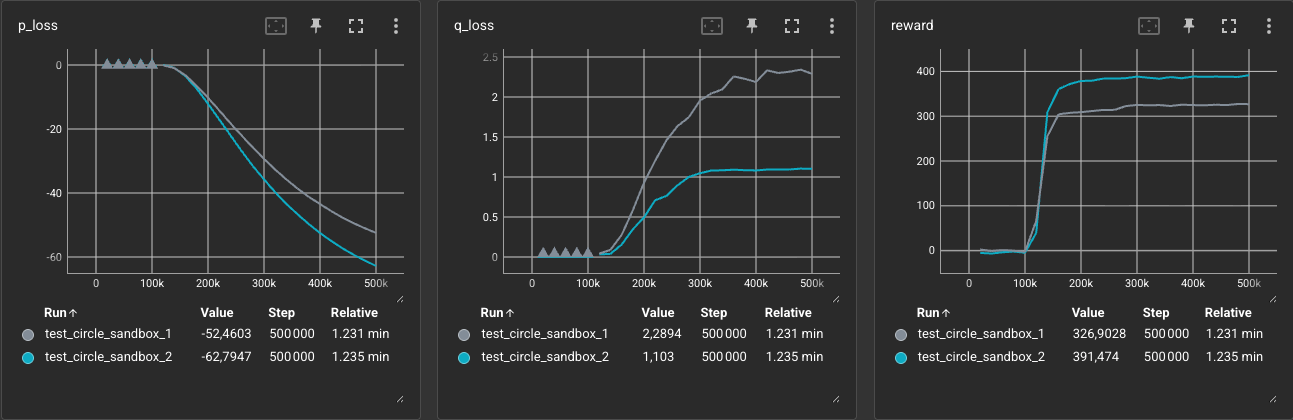
We notice a jump in accumulated reward from 327 to 391, as well as a more stable and lower q_loss (the Critic loss) from ~2.3 to ~1.1. Having access to its own velocity and predicting the leader’s next position allowed the agent to brake, anticipate turns, and stay closer to the leader.
Next Step: Let’s add a bit of complexity! Can the agent switch between tracking the leader and an environmental landmark, with the landmark becoming active at a random time?

4.2. Single Agent with Active Landmark (Exp. 3 & 4)

In this second phase, we introduce environment landmarks (goals) and increase the number of learning agents. This transitions the task from simple tracking to multi-point navigation.

4.2. Experiment 3: Dynamic Landmark Targeting

Goal: Follow the leader, but immediately switch to the landmark (goal_0) if it becomes active.
Reward:
- If goal_0 is active: $-\ln(\text{dist}(\text{agent}, \text{goal}_0))$
- If goal_0 is inactive: $-\ln(\text{dist}(\text{agent}, \text{leader}))$
Observation Space (7 dimensions):
- Agent’s own velocity: vx, vy
- Same offset to leader as in Exp. 2: dx, dy
- Offset to goal:
```
dx_goal, dy_goal = goal.x - agent.x, goal.y - agent.y
```
- Goal activation state: 1 if active, 0 otherwise.
Results: The agent successfully learned to switch targets depending on the goal’s activation state: it tracks the leader when the goal is inactive, and redirects to the goal when it becomes active.

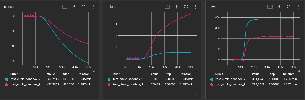
The reward was harder to accumulate, probably due to the travel time between the goal and the leader, but the agent learned to switch targets reliably.
Next Step: Let’s hypothesize: can we observe boids-like behaviors² (separation, alignment, and cohesion) emerge from simple rewards and observations? Can we try to encourage separation in the next experiment?

4.2. Experiment 4: Lag Position Estimation

Goal: Similar to Exp. 3, but follow an estimated lagged position behind the leader to see if a “separation” behavior would emerge.
Reward: Uses the same active/inactive goal reward logic, but the leader tracking target position is estimated using estimate_target_pos_2, which projects backwards based on the leader’s previous velocity:
```
return leader.p_pos - (leader.p_vel * coef) # coef=4.0 
```
We can see the coef as a projection to the past position of the leader, based on its velocity. If the leader keeps its velocity, it would be at the position p_pos - (p_vel * coef) at the current time step. Here coef=4.0 means we are projecting the leader to the position 4 time steps in the past.
Observation Space (7 dimensions): Similar to Experiment 3, but the relative offset to the leader is direct: dx, dy = leader.x - agent.x, leader.y - agent.y. (It is also “cheaper” to compute compared to Exp. 3.)
Results: By targeting a lagged position, the agent learned to maintain a natural tailing distance behind the leader rather than attempting to overlap with it, improving tracking smoothness.

The critic loss for Exp. 4 (~5.0) is significantly lower than Exp. 3 (~7.7). This is because in Exp. 3, the agent is trying to shadow the leader directly (overlapping). Since we use an unbounded log reward function, this creates high-frequency adjustments, overshoots, and erratic transitions, making it very hard for the Critic to predict future rewards.

In Exp. 3, we have a final accumulated reward higher than in Exp. 4 (220 vs 201). In Exp. 3, the agent sometimes overlaps the leader, which yields huge logarithmic reward spikes.

To be honest, it is difficult to say whether the agent performs better overall than in Exp. 3. While Exp. 4 exhibits a lower critic loss—indicating more stable training—the behavior visually appears more jittery.

4.3. Alignment and Complex Multi-Agent Dynamics (Exp. 5, 6 & 7)

In this new phase, we’ll introduce alignment, rewarding agents for matching the velocity and angle of their targets. For the separation behavior, we set the previous agent as the target for each agent. So we have a chain of agents, where each agent follows the previous one. We also choose to return the Exp. 3 reward function:

\[R_i = \begin{cases} -\ln \left( \|\mathbf{x}_i - \mathbf{g}_{i-1}\| \right), & \text{if } g_{i-1} \text{ is active,} \\ -\ln \left( \|\mathbf{x}_i - \mathbf{x}_{i-1}\| \right), & \text{otherwise} \end{cases}\]

Each agent follows either its assigned landmark (if active) or the previous agent (if inactive).

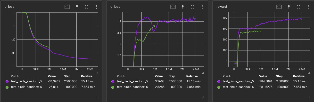
4.3. Experiment 5: Multi-Agent Chain Following (Leader-Follower-Follower)

Goal: This experiment extends Exp. 3 by introducing a third agent, establishing a 3-agent chain where Agent 1 follows the Leader (Agent 0) or goal_0, and Agent 2 follows Agent 1 or goal_1. To allow the policy to converge, we set the training time to 25,000 episodes instead of 5,000.
Reward:
- Agent 1: Proximity to goal_0 (if active) or estimated position of Agent 0 (if inactive).
- Agent 2: Proximity to goal_1 (if active) or estimated position of Agent 1 (if inactive).
Observation Space: 9 dimensions per agent:
- Agent’s own velocity: vx, vy
- Relative offset to target agent:
```
dx_target, dy_target = target.x - agent.x, target.y - agent.y
```
- Velocity of target agent: vx_target, vy_target
- Relative offset to assigned goal:
```
dx_goal, dy_goal = goal.x - agent.x, goal.y - agent.y
```
- Assigned goal activation state: 1 if active, 0 otherwise.
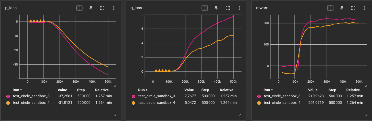
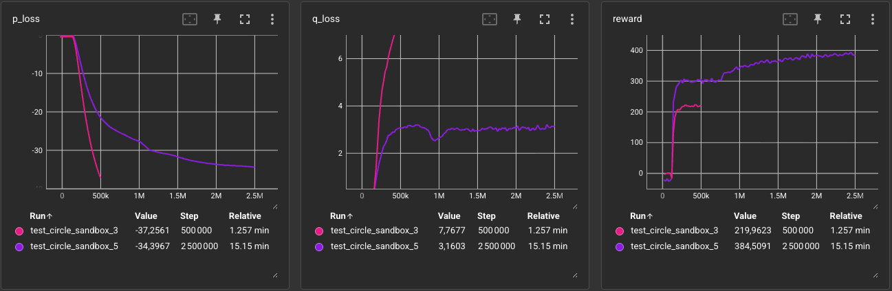
Results: The agents successfully learned chain-following behaviors. However, because they only observed their immediate target and goal (partial observability), any perturbation in Agent 1’s trajectory propagated downstream to Agent 2. We also observed one or two collisions per simulation between the two learning agents.

Note: In the environment, we increased the global collision response (from 100 to 500) to make interactions bouncier. Unfortunately, this also represents a greater penalty for colliding agents.

We notice key differences in this new training dynamic:
1. The total accumulated reward is higher because we sum the contributions of two learning agents; this averages 192 per agent, which is lower than the 219 achieved in Exp. 3, even after five times as many training steps.
2. Despite the added complexity, the Critic Loss (q_loss) is much more stable (3.1 vs 7.7)!
3. Exp. 5 takes much longer (around 2M steps) to fully mature and stabilize its policy loss (p_loss) compared to Exp. 3 (which drops quickly before 500k steps).
4. We observed some strange behaviors: the agents sometimes appeared to “wait” for a landmark to activate. This might be a sign of overfitting, where, given the predictable position of the Leader (a simple circling linear motion), the agents learned to wait for a spot to activate to get a higher reward. We see evidence of this in the reward curve, which plateaus around 300 and then rises again after 1M steps.
Next step: To avoid such overfitting, we will try reducing the number of training episodes. We’ll also continue our focus on alignment behavior.

4.3. Experiment 6: Chain Following with Velocity Alignment

Goal: Solve the chain-following task (3 agents, 2 landmarks) while smoothing out trajectories using velocity alignment.
Reward:

\[R_i = \begin{cases} -\ln \left( \|\mathbf{x}_i - \mathbf{g}_{i-1}\| \right), & \text{if } g_{i-1} \text{ is active,} \\ 0.7 \cdot \left( -\ln \left( \|\mathbf{x}_i - \mathbf{x}_{i-1}\| \right) \right) + 0.3 \cdot \max \left( 0, \text{cos_sim}(\mathbf{v}_i, \mathbf{v}_{i-1}) \right), & \text{otherwise} \end{cases}\]

where cos_sim is the cosine similarity, measuring how closely the agent’s velocity vector $v_i$ aligns with the target’s velocity vector $v_{i-1}$.

Observation Space (9 dimensions): Same as Experiment 5.
Results: The introduction of velocity alignment significantly improved path smoothness. The agents seem to have learned to match the heading of their targets, reducing large collisions, though some minor collisions still occur.

Comparing the training dynamics of Exp. 5 and Exp. 6, we can observe three key points:
1. Lower overall reward scale: The total accumulated reward in Exp. 6 is lower than in Exp. 5. This is a consequence of scaling down the proximity reward by 0.7 to make room for the 0.3 velocity alignment term.
2. Lower and more stable Critic Loss: The q_loss for Exp. 6 rises much more slowly and displays a notable dip to 2.1 around 500k steps (compared to Exp. 5’s peak of 3.2) before rising again. This temporary dip could occur when agents first master the velocity alignment, while the subsequent rise could correspond to learning the more complex landmark-switching behavior.
3. Reduced policy exploitation: By stopping the training at 1.0M steps in Exp. 6 (2.5M steps in Exp. 5), we successfully reduced the signs of policy exploitation (overfitting to the trajectory dynamics). The reward curve shows no evidence of multi-stage learning; the agents converge stably around a reward of 281 without discovering how to exploit the timing windows of the landmark activations to increase their score.
It is fascinating to see the q_loss reflect learning progress step-by-step!
Next step: Let’s try to see if it can scale to one more follower! We’ll add a bit more time to the simulation (20k episodes) and see how it goes.

4.3. Experiment 7: Chain Scaling (Leader + 3 Followers)

Goal: Scale the setup to 4 agents (1 leader, 3 followers) and 3 landmarks, establishing a longer chain where Agent 3 follows Agent 2.
Reward: Uses the same velocity alignment reward mix as Experiment 6.
Observation Space (9 dimensions per follower): Same as Experiment 6, mapping to their respective upstream target and assigned goal.
Results: This is a bit more… chaotic! Scaling the chain length significantly increased training difficulty. We can see delays in response propagated down the chain, as well as a lot of collisions.

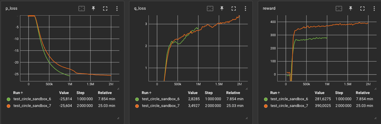
Comparing the training curves of Exp. 6 and Exp. 7 shows the clear cost of scaling the chain:
1. Drop in individual performance: The reward per agent drops from 141 to 130 (a 7.7% decrease), even with double the training time (2M steps).
2. The Whip Effect: This decline is caused by error propagation down the chain. Any minor correction or lag from Agent 1 is amplified downstream, leaving Agent 3 to deal with highly erratic target trajectories.
3. Increasing Critic Loss: The q_loss for Exp. 7 continues to climb, reaching 3.5 at 2M steps, reflecting the increased difficulty and non-stationarity of predicting transitions in a crowded, collision-prone chain.
Next steps:
1. To avoid underfitting, we’ll run the same experiment but with 100k episodes (5x more).
2. To avoid overfitting to a deterministic leader trajectory, we’ll add some randomness in the speed of the leader.
3. We’ll also try to encourage closer interaction by setting the same goal for all the agents. The hypothesis behind this is if the agents are forced to be at the same location, the “collision” case will be more present in their replay buffer, and they will likely learn more efficiently to avoid each other.

4.4. Longer Training and Reward Tuning (Exp. 8, 9 & 10)

This final phase addresses the instabilities and issues observed in previous experiments, while scaling training iterations up to 100k episodes (10M steps).

4.4. Experiment 8: Shared Same Active Goal

Goal: Solve the 4-agent chain-following task with 3 landmarks, but configure all learning agents to target the same last activated goal, instead of independent dedicated landmarks.
Reward: Same logarithmic-distance and velocity alignment mixture as Experiment 7.
Observation Space (9 dimensions):
- Local velocity: vx, vy
- Offset and velocity of the target agent: dx_target, dy_target, vx_target, vy_target
- Offset to the shared active landmark, and its activation state: dx_goal, dy_goal, 1 if active, 0 otherwise.
Results: On the bright side, transitioning to a shared active goal simplified the navigation logic. On the other hand, as anticipated, it introduced even more chaos.

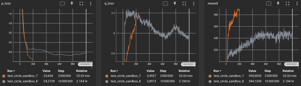
Comparing the training curves of Exp. 7 and Exp. 8 shows the physical impact of a shared goal:
1. The Crowding Penalty: The total accumulated reward is lower in Exp. 8 (349 vs 390). Since all three followers are heading to the same active goal simultaneously, they create a traffic jam at the goal. Bouncing off one another constantly prevents them from occupying the landmark space cleanly, dragging down the reward.
2. Critic Convergence over 10M Steps: Training for 10M steps allowed the Critic’s prediction error (q_loss) to stabilize to 2.89 (vs 3.5). This shows the Critics learned to model the high-collision states with high accuracy, but the Actor exploited the log reward, creating behavior where colliding with others could potentially lead to a peak of high rewards.
Next step: Our logarithmic reward function is suboptimal: it creates instability when agents approach the same active goal too closely.

To fix this, we could use a more stable reward mapping: a Bounded Exponential Decay, mapping error scales to a smooth $[0, 1]$ interval instead of the negative logarithm.

Comparing Negative Log vs Bounded Exponential Decay Rewards

Log Reward Instability and Domain Errors

As the distance reward approaches zero, $-\ln(x) \to +\infty$.

In practice, if an agent perfectly matches the target position, math.log(0) will throw a ValueError: math domain error and crash the training.

Even if it gets extremely close without reaching exactly zero, the reward explodes to a very large positive number, incentivizing the agent to exploit this reward to farm infinite values rather than focus on reaching its target.

Here is an example of how the Bounded Exponential Decay could be applied to the reward function:

  # sigma parameters control how quickly the reward drops off
  sigma = 1

  dist = dist(self.pos, target_pos)
  # distance reward is strictly bounded between [0, 1]
  r_dist = math.exp(-dist / sigma)
  # other rewards are also bounded between [0, 1]
  r_angle = min(0, cos_sim(self.vel, target_vel))
  
  # Weighted sum (maximum reward possible is 1.0)
  reward = 0.7 * r_dist + 0.3 * r_angle

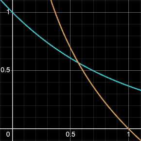Rewards comparison In yellow, the actual $-ln(x)$ on the interval [0, 1]. The more the error is close to 0, the more the reward explodes. In blue, the exponential decay $exp(-x)$ (when sigma = 1) on the interval [0, 1], the maximum reward possible is 1.0.

4.4. Experiment 9: Bounded Exponential Decay Rewards

Goal: Eliminate log-domain errors and instability by replacing the negative log function with a bounded exponential decay reward.
Observation Space (7 dimensions): Refined to use relative velocities expressed as signed angle differences and magnitude differences rather than raw Cartesian velocities:
- Relative offset to target: dx_target, dy_target
- Target-agent relative velocity: dv_angle, dv_mag
- Relative offset to shared active goal: dx_goal, dy_goal
- Goal active flag: 0 or 1.
Results:

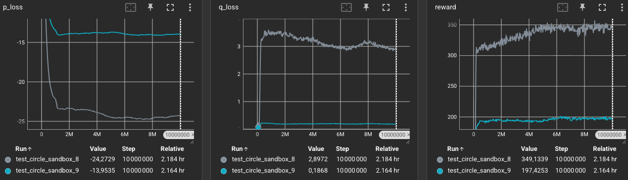
Comparing the training curves of Exp. 8 and Exp. 9 shows the dramatic stabilizing effect of switching to bounded rewards:
1. Normalized Reward Scale: The raw accumulated reward is lower (197 vs 349) simply due to the new reward bounds. In Exp. 9, the reward is capped at a theoretical maximum of 300 (100 steps * 3 agents). An average reward of 197 indicates that the agents are maintaining an excellent average proximity score of 0.66 out of 1.0 per step.
2. Collapse in Critic Loss Scale: Due to the change in the reward function, the Critic loss drops dramatically. The q_loss drops from an average of 2.9 in Exp. 8 down to under 0.19 in Exp. 9.
Since rewards were strictly bounded in the $[0, 1]$ interval, policy gradients were smooth, and agent oscillations were almost completely eliminated.
Next step: Let’s continue to improve the cohesion of our agents and give them the whole picture of the positions and velocities of all their neighbors. In practice, because we only have a few agents, we give them access to all other agents’ positions and velocities; however, in theory, we could restrict this to only the ones in the neighborhood of each agent.

4.4. Experiment 10: Larger Observation Space

Goal: Test the robustness of the policy by introducing all the positions and velocities for the agents’ observations. The idea is to introduce cohesion with the other agents of the “flock” and avoid collisions.
Observation Space: In addition to the offset and the relative velocity to the shared target and the shared goal, we add the relative offset and relative velocity to the other agents.
- Relative offset to target: dx_target, dy_target
- Target-agent relative velocity: dv_angle, dv_mag
Results:

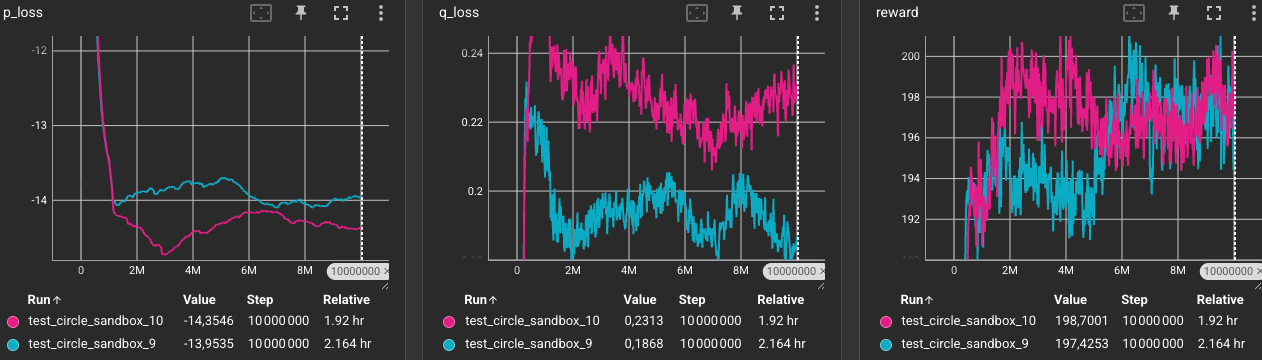
Comparing the training dynamics of Exp. 9 and Exp. 10 shows:
1. The Critic Loss (q_loss) moved from 0.18 to 0.24, a bit higher than in Exp. 9, likely due to the increased complexity introduced by considering other agents’ positions and velocities.
2. The rewards are very comparable (199 vs 197), meaning both setups achieve similar tracking performance.
3. The Policy Loss (p_loss) drops faster early on and converges to a more negative value in Exp. 10 (-14.35 vs -13.95). Since the policy loss represents the negative expected Q-value ($-Q$), this indicates that having access to neighbors’ positions and velocities allows the Actor to find high-value coordination strategies faster, with the Critic predicting higher long-term expected returns due to reduced collision interference! 🎉

4.5. Experiment Summary & Results

Exp.	Objective / Description	Observation Space	Reward Formulation	Training Length (ep.)	Acc. Reward
1	Single follower tracking a circular leader	Target relative position ($dx, dy$)	Logarithmic distance: $-\ln(d)$	5k	327
2	Follower learning smooth matching	Target $dx, dy$ + follower velocity	Same	5k	391
3	Single follower + 1 active/inactive goal	Same + goal (dx, dy, state)	Log. dist. to target or goal	5k	220
4	Single follower + leader future position estimation	Same as Exp. 3	Logarithmic distance to estimated future position	5k	201
5	Chain of 2 followers + 2 active/inactive goals	Same as Exp. 3	Same as Exp. 3	25k	385
6	Chain of 2 followers + velocity alignment reward	Target $dx, dy$ + goal info + velocity differences	Weighted: $0.7 \cdot \text{distance}$ + $0.3 \cdot \text{cos-sim}(v_{\text{agent}}, v_{\text{target}})$	10k	282
7	Chain of 3 followers + 3 goals + chain velocity alignment	Same as Exp. 6	Same as Exp. 6	20k	390
8	Chain of 3 followers + 3 goals + shared active goal	Local velocity + active goal offset & state	Same as Exp. 6	100k	349
9	Chain of 3 followers + 3 goals + Bounded Exponential Decay rewards	Relative velocity (angle/magnitude) + target & active goal offsets	Weighted: $0.7 \cdot e^{-d/\sigma_d}$ + $0.3 \cdot \text{angle_difference}$	100k	197
10	Chain of 3 followers + 3 goals + mutual agent collision awareness	Same as Exp. 9 + other agents’ relative offsets & velocities	Same as Exp. 9	100k	199

target: the leader or the previous agent in the chain.

dx, dy: target position - agent position.

Acc. Reward: shows the accumulated rewards for all agents (which can be divided by the number of agents to get the average accumulated reward per agent).

Max Theoretical Reward: Unbounded for log-based reward functions (Experiments 1–8) since $-\ln(d) \to +\infty$ as $d \to 0$. For Exp. 9 & 10, the reward function is bounded between 0 and 1 per step per agent, giving a strict maximum of $1.0 \times 100 \text{ steps} \times 3 \text{ followers} = 300.0$.

4.6 Under the Hood: Observations and Rewards

Crafting the observation space and the reward function is where the real RL magic (and frustration) happens.

For observations, each agent needs to know the relative distance to its target (d_pos), the difference in their velocities (dv_angle, dv_mag), and the state of their specific landmark. Here is a snippet from my 10th experiment:

"""Builds local observation representation for an agent."""
d_pos, lm_d_pos = (
    np.array([0, 0]),
    np.array([0, 0]),
)
dv_mag, dv_angle, lm_act = 0, 0, 0

# current agent velocity
vx = agent.state.p_vel[0]
vy = agent.state.p_vel[1]

# target distance
target_id = agent.id - 1
target = self.find_agent_by_id(world, target_id)
if target:
    self.fix_agent_vel(target)
    # delta x/y
    d_pos = target.state.p_pos - agent.state.p_pos
    # delta vel (signed angle and magnitude)
    dv_angle, dv_mag = self.get_angle_signed_and_mag(
        target.state.p_vel, agent.state.p_vel
    )

# active landmark
lm = self.get_last_active_landmark(world)
if lm:
    lm_d_pos = lm.state.p_pos - agent.state.p_pos
    lm_act = int(lm.activate)

# relative positions of other agents (excluding leader and target agent)
other_d_pos = []
other_d_vel = []
for other in world.agents:
    if other.id == 0 or other.id == agent.id or other.id == target_id:
        continue
    other_d_pos.append(other.state.p_pos - agent.state.p_pos)
    other_d_vel.append(
        self.get_angle_signed_and_mag(other.state.p_vel, agent.state.p_vel)
    )

# return the complete state
base_obs = [
    vx,
    vy,
    d_pos[0],
    d_pos[1],
    dv_angle,
    dv_mag,
    lm_d_pos[0],
    lm_d_pos[1],
    lm_act,
]
for dp in other_d_pos:
    base_obs.append(dp[0])
    base_obs.append(dp[1])
for dv in other_d_vel:
    base_obs.append(dv[0])
    base_obs.append(dv[1])

return np.array(base_obs)

For the reward function, balancing multiple objectives (distance, separation, and alignment) was challenging. We ultimately opted for logarithmic decay to heavily penalize agents when they were too far off track:

"""compute the reward for one agent"""
base_reward = 0.0
# scale param
sigma_d = 1.0

# if there is an active goal, reward the agent for being close to it
landmark = self.get_last_active_landmark(world)
if landmark:
    d = self.dist(agent.state.p_pos, landmark.state.p_pos)
    base_reward = np.exp(-d / sigma_d)

# else follow the previous agent 
else:
    target_id = agent.id - 1
    target = self.find_agent_by_id(world, target_id)
    target_pos = self.estimate_target_pos(agent, target)
    d = self.dist(agent.state.p_pos, target_pos)
    r_dist = np.exp(-d / sigma_d)
    cos_sim = max(0, self.cos_sim(target.state.p_vel, agent.state.p_vel))
    base_reward = 0.7 * r_dist + 0.3 * cos_sim

return base_reward

5. Learnings and Challenges

So, how did they learn?

Complexity kills convergence: Unsurprisingly, going from single-agent setups to multi-agent setups drastically increased convergence time.
Constraints cause instability: Introducing separation and alignment constraints resulted in high instability during training. When all constraints were applied at once, the agents struggled heavily to balance the trade-offs.
Environment & Compatibility Issues : Setting up this legacy RL codebase natively on MacOS ARM64 (Apple Silicon) presented several issues.

Compatibility Issues with Apple Silicon MacOS ARM64

Python Environment & Package Pinnings: Migrating the codebase to a modern uv workspace allowed managing Python 3.9/3.10 and the local subprojects (maddpg and multiagent) cleanly in editable mode. However, several strict version pins were required:
- numpy<2 (1.26.4): Prevented binary compatibility errors with TensorFlow 2.14.0.
- setuptools<70 (69.5.1): Retained pkg_resources which has been completely removed in modern setuptools but is still imported by legacy gym==0.10.5.
- pyglet==1.5.27: Pyglet 2.x drops support for legacy OpenGL 1.x/2.x functions (such as glPushMatrix, glPopMatrix, glBegin, etc.) which the MPE rendering engine heavily relies on. Pinning to 1.5.27 preserves legacy OpenGL compatibility.
Keras Cache Directory: In restricted or sandbox environments, Keras attempts to write to the protected ~/.keras directory. This was resolved by setting the environment variable KERAS_HOME=./.keras to redirect cache files to the workspace.
TensorFlow 2 Placeholder Bug: Under TensorFlow 2, symbolic placeholders are of class SymbolicTensor rather than the base tf.Tensor. A strict type check in tf_util.py (type(x) is tf.Tensor) failed to identify placeholders and silently stripped them from the execution feed dictionary, resulting in InvalidArgumentError: You must feed a value.... Updating this to isinstance(x, tf.Tensor) fully resolved the graph execution error.
Checkpoint Directory Loading Error: The load_state utility originally passed directory paths (e.g. ./test_circle_sandbox_9/best_model/) directly to saver.restore(), causing a FAILED_PRECONDITION: Is a directory error. We updated tf_util.py to check if the path is a directory and resolve the correct checkpoint prefix using tf.train.latest_checkpoint(fname).
OpenGL Line Width Exception: The 2D rendering engine called glLineWidth() with values greater than 1.0. Modern macOS graphics drivers throw a GLException: (0x1281): Invalid value when line widths greater than 1.0 are requested in certain profiles. We patched rendering.py to bound this call to 1.0 and gracefully handle any exceptions.

Final Conclusion

Over our 10 incremental experiments, we explored how observation representation, reward structure, and cooperative goals impact Multi-Agent Reinforcement Learning using MADDPG.

The key takeaways from this exploration are:

The Power of Centralized Training with Decentralized Execution (CTDE): Training a centralized Critic that sees all agents’ observations and actions effectively solves the non-stationarity problem. Once trained, the decentralization of the actors enables independent, real-time control based solely on local sensors.
The Criticality of Reward Design: Unbounded logarithmic rewards ($-\ln(d)$) are mathematically unstable when agents overlap perfectly, causing gradient explosion or software crashes. Switching to Bounded Exponential Decay ($e^{-d / \sigma}$) maps physical errors to a clean $[0, 1]$ interval, which stabilizes learning gradients.
Local Reference Frames Matter: Exposing relative angles and velocities rather than raw global values helps agents generalized coordination behaviors (like chain and circular tracking) much faster.
Coordination Bottlenecks: Scaling multi-agent chains introduces delay propagation (the “whip effect”), which can be mitigated by tracking the leader directly or allocating cooperative tasks dynamically (like shared active goals).
Emergence of Boids-like Behaviors: The classic rules of flocking (separation, alignment, and cohesion) seem to be able to emerge from reinforcement learning. By structuring reward functions to balance proximity and velocity alignment, we observed coordinated collective behaviors without hardcoding explicit swarm pathing.

What’s Next?

This project was a great dive into the world of MARL, but there is still plenty to do:

Alternative Observation: In our last experiment, we used all the global information possible for each agent. Next, we will try to limit the amount of information available to each agent to only their local neighbors to test if they can learn to coordinate with limited information. We will also try to average the position of the neighboring agents to keep the observation state from being too large.
Introduce Obstacles: Adding static or moving obstacles will force the agents to learn dynamic pathing on top of their current coordination and tracking constraints.
Longer Training: In the complex multi-objective scenarios, we could continue to train for a longer time to see if the chain instabilities eventually smooth out (particularly the last scenario).

Thank you for reading and stay tuned for more updates as we continue to experiment with these particle swarms!

In Temporal Difference (TD) learning, an agent updates its value estimates based on the difference between successive predictions of the value function. At each time step, the agent observes a reward and estimates the value of the next state. The TD error measures how far off the current prediction is from this new estimate, and the value function is updated to reduce this error. In practice, storing these transitions in an experience replay buffer allows the agent to observe and learn from rewards collected over time. TD learning is a core concept in reinforcement learning that allows agents to learn from experience without needing a full model of the environment. ↩
Boids² is a classic simulation of collective behavior, where simple autonomous agents (boids) interact locally with their neighbors according to three rules: Separation (avoid crowding), Alignment (match velocities), and Cohesion (steer toward the center of the flock). Despite the simplicity of these rules and the absence of global coordination or higher-level intelligence, these agents collectively produce complex, emergent group behaviors—such as flocking, swirling, and navigating around obstacles—that resemble the behavior of real bird flocks. Reynolds, C. W. (1987) Flocks, Herds, and Schools: A Distributed Behavioral Model, in Computer Graphics, 21(4) (SIGGRAPH ‘87 Conference Proceedings) pages 25-34. ↩